01Can gradient alignment make supervision on-policy? Rollout·NOV 2026
01Can gradient alignment make supervision on-policy? Rollout·NOV 2026
Claude Code v2.1.159 released, adopting a gradient alignment reward mechanism, using the Qwen3-8B model on arithmetic tasks, rewarding by calculating the gradient similarity between student output and expert demonstrations, experiments show the model may overfit the precise wording of expert examples.
Figure 1
Introduction
When looking to post-train a model, we can divide methods broadly into two axes: where we take our gradients from and where our learning signal comes from. Placing this perspective on classic post-training, supervised fine-tuning (SFT) or next-token prediction on a given set of demonstrations, gets gradients and also learning signal from these “expert” demonstrations. In contrast, RL receives gradients from the student’s own samples and then receives the learning signal from a reward. Both methods serve their own purpose and offer some clear tradeoffs:
1. SFT can add more information into the model directly (either through data or a teacher), but can often erode base capability.
2. RL can enable learning while keeping base capabilities, but is limited by both (a) what the model can already feasibly solve, and (b) a reliable reward structure.
This context leads us to a natural question: is it possible to keep expert demonstrations as the source of the learning signal whilst still taking gradients on student samples? This would require a reward function definable from an arbitrary dataset or teacher model, which would in theory offer the benefits of on-policy RL while also providing the generality of SFT. Last week we explored OPSD, another promised best-of-both-worlds algorithm, where we found that its bias can still behave more like SFT and shift model behavior (article link). This week, in an effort to go even closer to standard on-policy RL, we shift our attention to a closely related cousin, gradient alignment rewards.
Gradient alignment reward
Gradient alignment rewards [1, 2, 3, 4, 5, 6, 7] have been reintroduced more recently as a method for scoring a student rollout against an expert demonstration. This is achieved by converting both the student rollouts and expert demonstrations to the same shape via their log-likelihood gradients.
Let qθ be the student model, x a prompt, and y⋆ an expert demonstration. Define the expert and student rollout gradients as
gθ⋆=∇θlogqθ(y⋆∣x),gθ(y)=∇θlogqθ(y∣x),y∼qθ(⋅∣x).
We then assign the reward
rθ(x,y,y⋆)=⟨gθ(y),gθ⋆⟩∥gθ(y)∥ ∥gθ⋆∥
with numerical stabilization when either norm is close to zero.
gb:=gθ(yb),rb:=rθ(x,yb,y⋆),Δθ=η∇θ[1B∑b=1Bstopgrad(rb)logqθ(yb∣x)]=ηB∑b=1Brbgb.
There are a few ways we can view this reward. One is geometrically, from the gradient structure: when writing the full gradient update, we get a weighted sum of projections of the expert gradient onto individual rollout gradients:
Δθ=ηB∥gθ⋆∥∑b=1Bgbgb⊤∥gb∥ gθ⋆=ηB∥gθ⋆∥∑b=1B∥gb∥ projspan{gb}(gθ⋆).
We can also view this from the statistical point of view, using the implicit loss function approximation. Note that for a small step size η, we get the following Taylor approximation:
logqθ+ηgθ⋆(y∣x)qθ(y∣x)≈η⟨gθ(y),gθ⋆⟩,
The RHS is our (unnormalized) gradient alignment reward, and the LHS is a self-distillation-style likelihood ratio [8, 9], but instead of putting the expert example into context, we take a small gradient step towards increasing likelihood on the expert example. This latter interpretation starts to highlight some of the behavior we end up seeing: namely, that this reward can still notably bias towards the exact wording of expert examples in the same way SFT does.
Computing the reward at scale
There’s an important bottleneck above that makes a naive implementation computationally infeasible: materializing each individual batch elements’ gradient, which are typically summed over in a standard backward pass. This has led to this alignment reward being approximated or truncated; for example by considering only the output layer [4, 7]. However, using some tensor tricks and linearity, we can actually compute the full reward quite efficiently: effectively two standard backward passes! As this is purely on the trainer side (while rollouts are typically the compute bottleneck), this in practice adds little overhead.
To illustrate, we work through a single linear layer W by hand, and focus on just the inner products ⟨gθ(y),gθ⋆⟩; other layer types and the needed batch-gradient grad-norms follow similarly.
Let W have din input and dout output dimensions, with b=1,…,B indexing rollout sequences and t=1,…,T indexing tokens. For sequence b, Ab is the T-by-din matrix of input activations and Db is the T-by-dout matrix of derivatives of logqθ(yb∣x) with respect to the layer outputs; the individual weight gradient gb and the usual batch-summed weight gradient are:
gb=∇Wlogqθ(yb∣x)=Db⊤Ab,∇W∑b=1Blogqθ(yb∣x)=∑b=1BDb⊤Ab.
Ordinary backpropagation contracts the token and batch axes, leaving one matrix indexed by input and output features. However, by linearity, we can instead contract feature dimensions first and tokens last, leaving one scalar per sequence:
⟨gb,gθ⋆⟩F=⟨Db⊤Ab,gθ⋆⟩F=⟨Db,Ab(gθ⋆)⊤⟩F=∑t=1T⟨Db[t,:], (Ab(gθ⋆)⊤)[t,:]⟩.
Storing gθ⋆ takes one weight-sized matrix, so including its computation, total time and layer storage have the same asymptotic bounds as the base backward pass, with constant-factor overhead:
Normal backpropagationGradient alignment scoresTimeO(BTdindout)O(BTdindout)SpaceO (dindout+BT(din+dout))O (dindout+BT(din+dout))
These alignment scores are then used to compute the final gradient, for the second standard backward pass that scales each input gradient batch element by the now-computed cosine similarities.
Can the model still overfit?
All experiments are on four-number Countdown, using Qwen3-8B as the base model, to test the effectiveness of expert-provided rewards in an environment where verifiable rewards exist. Expert rollouts were generated by Opus 5.5.
Before we train at a broader scale, we first test a toy example using a single prompt and demonstration. First, we ask whether doing RL on the gradient alignment reward can fit at all. Second, we then ask if it will overfit to exact wordings in the same way as SFT would. As hinted at with the Taylor approximation interpretation, we would expect that it would.
Investigating these questions, we see the (a) accuracy rises to 100% within 100 updates, so the reward is consistent and we can learn, and (b) by update 100 all 64 samples are identical (reproducing the expert solution word for word) (Figure 1).
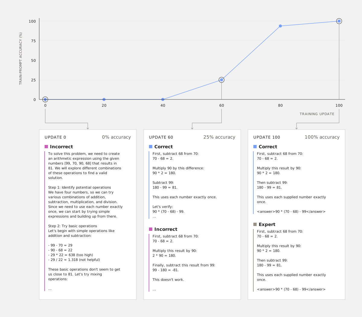
Figure 2
Optimizing gradient alignment rewards over a single prompt and expert demonstration. There is an initial learning phase where the model picks up on the expert pattern, but eventually overfits so that all rollouts match the expert wording exactly.
The intuition here is that the “reward” scores each rollout against the student after a single SFT step on the expert demonstration, meaning that we expect the wording of the demonstration to be evident in the reward.
How useful is the gradient alignment signal then?
We know that we’re able to train on this signal, but how well does this align with the actual environment rewards? While we do not expect this to be noiseless and perfectly correlated, we would hope that numerically correct answers correspond to higher gradient alignment rewards. Unfortunately, this separation is quite small, as can be seen by Figure 2.
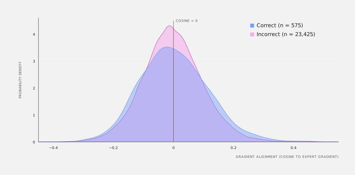
Figure 3
Distribution of gradient alignments, shown separately for correct and incorrect answers. Curves are kernel density estimates with Gaussian kernels (not fitted Gaussians). Notably, both distributions look fairly Gaussian, have similar means, with the correct responses having slightly higher variance.
While the two distributions are discernible in variation (and thus higher gradient alignment thresholds will have higher correct ratios), the initial reward structure makes it hard for this reward to get off the ground itself. The remaining question is if this provides any meaningful signal on top of a standard RL run, that standard baselines are unable to provide.
How well do gradient alignment rewards train?
While initial correlations to verified rewards are quite small, we know these rewards are trainable and can hope that through the training process, the gradient alignment rewards can become increasingly useful.
To this end, we compare the following methods on a smaller Countdown subset:
1. Purely using the gradient alignment reward from expert trajectories. As indicated by Figure 2, this reward alone is too noisy to make reliable gains on the underlying environment.
2. Gradient alignment in combination with verified rewards, which is the more common use case. One approach is to rely on gradient alignment rewards only when verified rewards provide little to no signal:
ri={cos(gi,gexpert),k<2,1[rollout i is correct],k≥2.
where k is the number of correct rollouts in a group size of 8. This provides some uplift, but is beaten by the following methods:
3. Standard GRPO with verified rewards (hyperparameters matched to best gradient alignment run), which is unsurprising given access to the true rewards, and finally:
4. SFT with a KL penalty over on-policy rollouts. As anticipated from the geometric interpretation, gradient alignment rewards can still behave like SFT iterates, and letting SFT steps go unconstrained can allow for easier optimization.
Results are all presented below in Table 1:
| Method | Validation accuracy | Correct / 256 |
|---|---|---|
| Base model (update 0) | 3.9% | 10 |
| Pure gradient alignment | 3.5% | 9 |
| Grad alignment + verified rewards | 10.9% | 28 |
| Verified rewards only | 23.4% | 60 |
| SFT + KL penalty | 20.3% | 52 |
Table 1: training results on a subset of Countdown. Evaluation comes from 256 held-out prompts.
Closing thoughts
Gradient alignment provides a way to use expert demonstrations while training on student-generated responses. Its reward changes with the student, and allows the algorithm to train purely on student rollouts, providing promise for an on-policy method for instilling knowledge into a student model.
However, this particular reward (a) is still able to overfit to specific examples, and (b) is a noisy estimate of correctness, and can be hard to train on. Notably the reward is strongly parameter-dependent, allowing for the model to hack it in stronger ways. These results are preliminary, and we don’t make any strong statements here on gradient alignment rewards and their utility, but as we like to say: great ideas are usually easier to get working.
References
1. M. Ren et al. Learning to Reweight Examples for Robust Deep Learning. PMLR 80:4334–4343, 2018.
2. S. Müller, A. Biedenkapp and F. Hutter. In-Loop Meta-Learning with Gradient-Alignment Reward. arXiv:2102.03275, 2021.
3. S. Li et al. LearnAlign: Data Selection for LLM Reinforcement Learning with Improved Gradient Alignment. arXiv:2506.11480, 2025.
4. Z. Liang et al. Can LLMs Guide Their Own Exploration? Gradient-Guided Reinforcement Learning for LLM Reasoning. arXiv:2512.15687, 2025.
5. Z. Zhang et al. Grad2Reward: From Sparse Judgment to Dense Rewards for Improving Open-Ended LLM Reasoning. arXiv:2602.01791, 2026.
6. N. Yang et al. GradAlign: Gradient-Aligned Data Selection for LLM Reinforcement Learning. arXiv:2602.21492, 2026.
7. L. Zheng et al. Gradients Know What Outcomes Don't: Unlocking Reinforcement Learning for LLM Reasoning with Gradient-Aligned Rewards. arXiv:2609.03342, 2026.
8. S. Zhao et al. Self-Distilled Reasoner: On-Policy Self-Distillation for Large Language Models. arXiv:2601.18734, 2026.
9. I. Shenfeld et al. Self-Distillation Enables Continual Learning. arXiv:2601.19897, 2026.
Source: Baseten Labs · labs.baseten.co