QDC 2026: what quantum developers need to know

Key takeaways:

• IBM Quantum Developer Conference 2026 (QDC 2026) unveiled a wave of new Qiskit tools for developers, spanning hardware, error correction, workloads, applications, and access.
• IBM Quantum Nighthawk r2, the fastest processor yet, gives developers direct pulse-level control for building, running, and iterating on frontier quantum circuits.
• New error-correction tooling lets developers build with fault-tolerant primitives today, from stabilizer-code frameworks to long-running repetition-code experiments on real IBM Quantum hardware.
• The directed execution model and new managed workflows on IBM Quantum Platform give developers more control while scaling across quantum and high-performance classical computing.
• Expanded application tooling connects real problems in chemistry, materials, and optimization to quantum circuits, turning verified quantum advantage into practical workflows.
• Every release pairs with IBM Quantum docs, tutorials, and runnable Qiskit code, plus new AI agent skills and expanded free access to start building.

Quantum advantage is increasingly a developer experience, not just a research milestone. That transition was on full display at IBM Quantum Developer Conference 2026 (QDC 2026), which showcased the practical tools that help developers build, test, optimize, and scale quantum workloads today.

Across the event, IBM highlighted a growing portfolio of Qiskit-based and community-driven tooling for exploring industry applications, contributing to open source, building production-ready workflows, and academic research. In this post, we’ll walk you through the releases that matter most for developers across hardware, software, error correction, and access—and we’ll show you how to get started building with each.

High-performance hardware for frontier circuits

For developers, everything starts with the hardware. This year, a big jump in speed made it easier than ever to build, run, and iterate on frontier quantum circuits that test the limits of our capabilities.

IBM Quantum Nighthawk r2 — developer capabilities

Our fastest processor (120 programmable qubits, up to 100,000 samples/sec), with pulse-level access developers can use directly: mid-circuit measurement, fast qubit reset, dynamic circuits, and soft (IQ) readout.

Why it matters: The speed and real-time control that make frontier circuits practical, plus the hooks to test error-correction techniques on real hardware today.

Get started: Read the Nighthawk r2 blog and run circuits today on IBM Quantum Platform.See what Nighthawk can do with our onset of ergodicity tutorial, which runs and analyzes a 64-qubit experiment on a Nighthawk processor.

Code: Speed is what lets you explore frontier circuits at scale—and you don't have to take our word for it. IBM's device benchmarks are all public, so you can measure a processor's max circuits per second (MCPS) yourself.

from qiskit_ibm_runtime import QiskitRuntimeService
from qiskit_device_benchmarking.mcps.mcps_benchmark import MCPSBenchmark

service = QiskitRuntimeService()
bench = MCPSBenchmark(service, "ibm_nighthawk")  # your backend name
print(bench.mcps())
# e.g. {'mcps': ..., 'num_circuits': 1000, 'shots': 1000, 'total_time_seconds': ...}

For a more hands-on test, the mirror benchmark runs a utility-scale circuit and checks its accuracy—part of IBM's fully open benchmarking suite (MCPS, CLOPS, EPLG, and more).

Enabling error correction research

Error correction was one of the most important themes at QDC 2026, with the quantum team showcasing an expanded error-correction stack. This included new developer tooling that lets developers begin working with the concepts, workflows, and abstractions that will underpin future error-corrected systems.

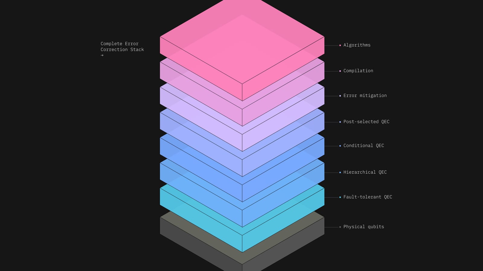
These tools are part of an integrated suite that spans the full stack. Alongside error-correction frameworks like Qiskit Paulice, you'll find modular error-mitigation tools—qiskit-mitigation and qiskit-noise-learning—covered later in this post in the “running and scaling workloads” section.

Qiskit Paulice

A framework supporting stabilizer-based computations and quantum error-correction workflows (spacetime codes for Clifford circuits).

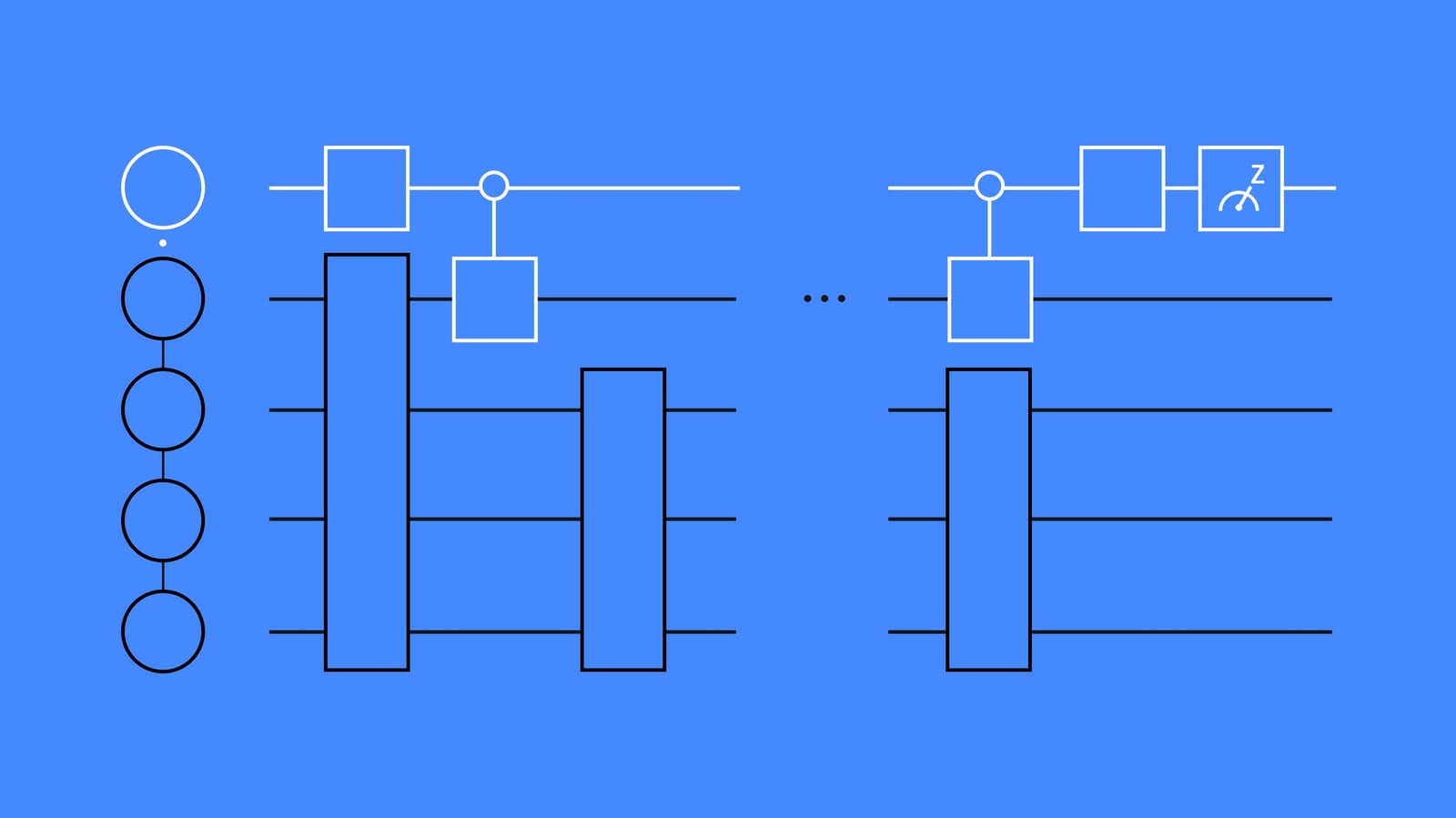
Why it matters: Lets developers and researchers start building with the primitives of fault-tolerant quantum computing today.

Get started: Read the Paulice blog, explore the docs, or work through the spacetime-codes tutorial on IBM Quantum Platform.

Code: Here's the core workflow—adding spacetime checks to a Clifford circuit to improve the fidelity of its measured distribution:

pip install qiskit-paulice

from qiskit import QuantumCircuit
from qiskit_ibm_runtime import QiskitRuntimeService
from qiskit_paulice.layout import get_check_qubits
from qiskit_paulice.noise_models import NoiseModel
from qiskit_paulice import add_pauli_checks

# Your Clifford circuit (here, a 12-qubit brickwork of entangling + single-qubit Clifford layers)

# Pick a device layout, then find target/ancilla qubit pairs from device connectivity
backend = QiskitRuntimeService().backend("ibm_boston")
layout = [68, 69, 78, 89, 90, 91, 98, 111, 112, 113, 119, 133]
target_qubits, ancilla_qubits = get_check_qubits(backend.coupling_map, layout)

# Build a depolarizing noise model from backend data to score candidate checks
noise_model = NoiseModel.from_backend(backend, layout)

# Search for effective, low-weight checks and add them to the circuit
checked_circuit = add_pauli_checks(
    circuit, [layout.index(q) for q in target_qubits], noise_model
)[-1]
# → a circuit with 7 checks, ready to run

From here, the Paulice documentation covers running the checked circuit, postselecting error-free samples, and comparing fidelities before and after.

Pulse-level capabilities

Error-correction research demands fine-grained control over what the hardware does and when. IBM Quantum Platform and the Qiskit software stack expose that control directly, rather than hiding it behind a black box. Three groups of capabilities do the heavy lifting:

• Real-time measurement and feedback. Dynamic circuits let researchers measure qubits mid-circuit and branch on the outcome in real time — the basis of syndrome extraction and feedback — using low-overhead instructions like MidCircuitMeasure.
• Precise timing control. You can set exactly when signals fire to protect idle qubits from noise, building custom dynamical decoupling sequences and shaping circuit timing through the transpiler's scheduling passes.
• Custom calibration. Beyond IBM's default calibrations, you can request instructions calibrated for a specific workload — including qec_experimental, the experimental default for the for_loop instruction behind the repetition-code experiment in the next section — or trigger a fresh calibration inside a session to counter drift during long runs.

For teams exploring soft decoders, raw IQ readout data — useful for leakage detection and confidence scoring — is also available by setting the measurement level.

Why it matters: Real codes only run when these capabilities work together, on hardware fast and large enough to exercise them. Having them directly accessible lets researchers develop, debug, and stress-test error-correction workflows on real devices today — not just in simulation. (Some, like in-session calibration and qec_experimental, are experimental and may change.)

Get started: Dynamic circuits and mid-circuit measurement are the best on-ramp — begin with the repetition codes or long-range entanglement tutorials. For timing control, see the scheduling guide; for drift during long runs, there's a new in-session calibration guide section.

Code: The repetition-code experiment that follows puts two of these capabilities to work directly — the experimental qec_experimental calibration and the MidCircuitMeasure instruction. For a single hands-on example that also brings in custom dynamical decoupling and advanced scheduling, work through the dc-hex-ising tutorial.

Repetition Code

We can now run a 1,000,000-round repetition code experiment end to end on IBM Quantum Platform. That’s a million mid-circuit measurement and reset layers in a single circuit. This is made possible by the for_loop instruction, which repeats a block of operations (including mid-circuit measurement) a fixed number of times without unrolling it into an enormous circuit.

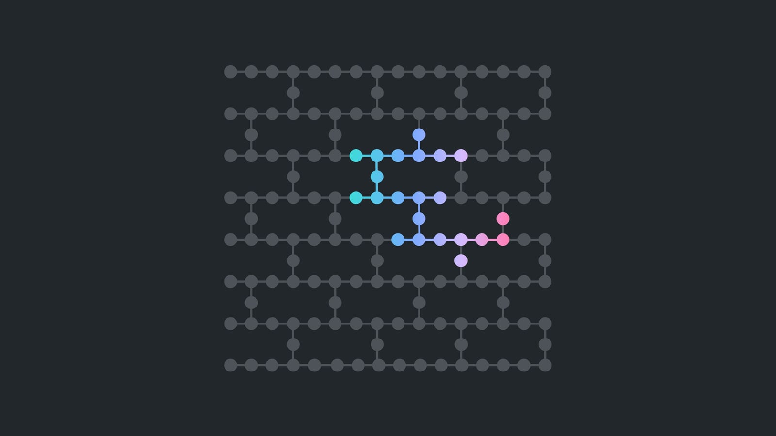
Why it matters: This is the kind of long-duration QEC workload you’ll need once logical error rates are very low—i.e., when error-corrected computations run for millions of rounds. Being able to execute it end to end today lets researchers develop and stress test those workflows on real hardware now.

Get started: See the custom calibration guide for the for_loop instruction and qec_experimental calibration. Note that both are experimental and may change. In particular, for_loop is currently supported only in Executor and client-side Sampler jobs.

Code: Here's the structure of a repetition-code experiment using for_loop—shown with 100 rounds to illustrate the pattern. The same circuit scales to the million-round run described above.

from qiskit import QuantumCircuit, QuantumRegister, ClassicalRegister
from qiskit import transpile
from qiskit.circuit.classical import expr, types
from qiskit_ibm_runtime import QiskitRuntimeService
from qiskit_ibm_runtime import Executor
from qiskit_ibm_runtime.quantum_program import QuantumProgram
from qiskit_ibm_runtime.circuit import MidCircuitMeasure

service = QiskitRuntimeService()
backend = service.backend("<backend_name>", calibration_id="qec_experimental")

num_data_qubits = 5
num_rounds = 100

data = QuantumRegister(num_data_qubits, "data")
ancilla = QuantumRegister(num_data_qubits - 1, "syndrome")

# Holds the current round's measurement results
cache = ClassicalRegister(num_data_qubits - 1, "cache")

# One register per syndrome qubit, one bit per round
checks = [
    ClassicalRegister(num_rounds, f"syndrome_{i}")
    for i in range(num_data_qubits - 1)
]

# Final readout of data qubits
final_data = ClassicalRegister(data.size, "data")

qc = QuantumCircuit(data, ancilla, cache, *checks, final_data)

with qc.for_loop(range(num_rounds), expr.Var.new("r", types.Uint(32))) as r:
    qc.barrier()
    for i in range(num_data_qubits - 1):
        qc.cx(data[i], ancilla[i])
    for i in range(num_data_qubits - 1):
        qc.cx(data[i + 1], ancilla[i])
    qc.barrier()
    for i in range(num_data_qubits - 1):
        qc.append(MidCircuitMeasure(), ancilla[i], cache[i])
        # Copy the result into this round's bit
        qc.store(expr.index(checks[i], r), cache[i])

# Measure data qubits
for i in range(num_data_qubits):
    qc.measure(data[i], final_data[i])

# Layout and transpilation
tqc = transpile(
    qc,
    backend,
    initial_layout=[0, 2, 4, 6, 8, 1, 3, 5, 7],
    optimization_level=0,
)

executor = Executor(mode=backend)
program = QuantumProgram(shots=10000)
program.append_circuit_item(tqc)
job = executor.run(program)
result = job.result()

# Boolean array with shape (shots, num_rounds)
syndrome_0 = result[0]["syndrome_0"]

Running and scaling workloads

As quantum workloads grow more sophisticated, execution and orchestration matter as much as the circuits themselves. This year’s releases give you more control over how a workload runs—without giving up performance—and more ways to scale it across quantum and classical resources. Updates to the IBM Quantum Platform usage and user experience also make quantum workloads more manageable and understandable, while Quantum Resource Management Interface (QRMI) strengthens the integration of quantum computing into high-performance computing workflows.

Workload estimation and expanding platform resources

New usage estimation tools on IBM Quantum Platform give users greater visibility into resource consumption before execution, helping them plan, optimize, and run workloads with confidence. The platform is also expanding to support a broader range of quantum and classical computing capabilities, enabling more sophisticated workflows.

To support these enhancements, IBM Quantum is introducing Resource Units (RUs), a unified capacity model across platform resources. For standard QPU workloads, 1 RU equals 1 minute of QPU compute time, so existing capacity and pricing carry over directly.

Why it matters: Know how much capacity your workload is expected to consume before execution, so you can optimize resource usage and experiment with confidence.

Get started: Explore our access plans and Resource Units overview, then learn how to estimate usage before you run.

Code: Estimate a workload’s usage without consuming any QPU time by performing a dry run:

service = QiskitRuntimeService()
backend = service.backend("<backend_name>")
executor = Executor(mode=backend)
job = executor.run(program, dry_run=True)
result = job.result()  # randomized mock data
usage = job.usage()    # estimated consumption

Use the estimate to right-size your experiment and check it against your allocation before submitting it.

Managed workflows

Premium and Flex plan users can deploy and run quantum-classical workflows on managed, high-performance classical infrastructure.

• Run your workflow on managed high-memory and GPU-accelerated compute. You can start large-scale parameter-sweeps on your laptop, and managed workflows complete and track the entire execution on IBM Quantum Platform.
• Fully managed environments. Your workflow is executed securely in a managed environment with the latest Qiskit tools. You can also bring your own wheels for custom packages, and save to persistent storage to store checkpoints between runs.
• End-to-end observability. View the entire execution lifecycle and underlying quantum + classical resources used per workload, directly in the workloads table.
• Pay for classical with resource units. You can run your workflow on several classical compute profiles, and pay per-second with resource units.

Why it matters: Deploy your quantum-classical workflow once and scale up with powerful classical compute environments beyond your laptop.

Get started: Learn how to deploy managed workflows by reading the documentation on IBM Quantum Platform, or use an AI skill to analyze and deploy your custom workflow.

IBM Quantum Functions Catalog

IBM Quantum Functions is now in Beta, with several new tools and improvements that make it easier for you to get real work done on IBM Quantum Platform:

• Manage errors with new circuit functions. Explore LTM's AI-QEM function and Quantum Elements' Orbit function—robust techniques to configure and run circuits at scale with minimal overhead.
• Solve optimization problems with three new application functions. Tackle constrained optimization with the Aqarios Constrained Quantum Optimizer, reduce depth and overhead with ParityQC's Parity Twine Optimizer, or go beyond 1:1 mapping with Jij's SQOASolver.
• Extract quantum features for ML pipelines. Add quantum feature extraction to your existing machine learning workflows with Kipu Quantum's Rimay function.
• Simulate quantum many-body dynamics. Model time evolution with Q-CTRL-powered dynamics simulation. Specify the physical model, initial state, time-evolution parameters, and observables, then retrieve a full time trace of expectation values.
• Pay per workload with a flexible new billing model. At launch, run Catalog Functions on a consumption-based model with no upfront commitment, billed per-workload using resource units in your Premium and Flex plan.

Why it matters: Leverage the latest research software tools from our ecosystem to accelerate applied research iterations, now without procurement hurdles.

Get started: Browse the IBM Quantum Functions catalog to see the full catalog of functions available, and add to your existing instance with a few clicks on the IBM Quantum Platform.

Samplomatic and Executor

Samplomatic builds twirled, annotated circuits, and Executor runs them with full control and transparency—no hidden error suppression. Together, these tools form the core of the directed execution model.

Why it matters: Add composable transformations like gate and measurement twirling, then run the result as a single program—repeatable, transparent workflows as you move beyond one-off demonstrations toward larger research or production-ready initiatives.

Get started: Read through the Samplomatic and Executor docs on IBM Quantum Platform.

Code: The following code example shows how to box and twirl a circuit with Samplomatic, package it as a quantum program, and run it with Executor.

from samplomatic.transpiler import generate_boxing_pass_manager
from samplomatic import build

from qiskit_ibm_runtime import Executor
from qiskit_ibm_runtime.quantum_program import QuantumProgram

# Generate a boxing pass manager to group gates
# and measurements into boxes and add
# a `Twirl` annotation.
boxes_pm = generate_boxing_pass_manager(
    enable_gates=True,  # Add gate twirling
    enable_measures=True,  # Add measurement twirling
)

boxed_circuit = boxes_pm.run(isa_circuit)

# Build the template circuit and the samplex
template_circuit, samplex = build(boxed_circuit)

# Append the template circuit and samplex as a `samplex_item`
program = QuantumProgram(shots=25)
program.append_samplex_item(
    template_circuit,
    samplex=samplex,
    shape=(num_randomizations := 20,),
)

executor = Executor(mode=backend)
job = executor.run(program)

The result is a twirled, annotation-driven execution you can reproduce and scale without giving up visibility into what ran.

Client-side Sampler and Estimator

New client-side Sampler and Estimator primitives run their pre- and post-processing—including error mitigation—on the client, delegating execution to the Executor. Because that logic lives in your environment instead of behind a server-side black box, you can inspect it, adjust it, or write your own methods against Executor directly.

Why it matters: Convenience when you want it, control when you need it. Applied researchers keep the familiar primitive interface, while anyone who needs fine-grained control can see and customize exactly what happens before a circuit runs. Local testing now applies the same error mitigation you'd get on hardware, so prototyping actually reflects real runs.

Get started: Work through the Get started with Sampler and Get started with Estimator docs on IBM Quantum Platform. Moving existing code over? See the migrate to client-side primitives guide—or let the migrate-qiskit-ibm-runtime AI skill handle it.

Code: To use the client-side primitives, simply import and run them just as you would the originals.

from qiskit_ibm_runtime.executor_sampler import Sampler
from qiskit_ibm_runtime.executor_estimator import Estimator
# On qiskit-ibm-runtime 0.52.0 or later, these imports
# can be simplified to:
# from qiskit_ibm_runtime import Sampler, Estimator

# Sample measurement outcomes from a circuit
sampler = Sampler(mode=backend)
job = sampler.run([(isa_circuit, param_values)])
result = job.result()

# Or estimate expectation values for an observable
estimator = Estimator(mode=backend)
job = estimator.run([(isa_circuit, isa_observable, param_values)])
expectation_values = job.result()[0].data.evs

Same interface, more transparency—the mitigation that used to be hidden server-side is now yours to inspect and extend.

qiskit-mitigation and qiskit-noise-learning

New, modular error-mitigation and Pauli-Lindblad noise-learning packages enabled by the directed execution model.

Why it matters: No more fixed, black-box pipelines. Compose and customize mitigation yourself—for example, by building postselected noise models to reduce PEC sampling overhead.

Get started: Explore the qiskit-mitigation and qiskit-noise-learning docs, and learn how to cut PEC sampling overhead with postselected noise models via our PEC with logical noise models tutorial.

Code: The full workflow is involved, so here's just the key step—after learning a Pauli-Lindblad noise model, then building a postselected mask that shrinks what PEC has to cancel. (This is illustrative, not runnable as-is; the PEC tutorial has the complete, runnable version.)

from qiskit_mitigation.noise import create_postselected_noise_mask

# After learning a Pauli-Lindblad noise model with qiskit-noise-learning,
# build a postselected mask that shrinks the noise model PEC must cancel
local_scales, gamma2_post = create_postselected_noise_mask(boxed, noise_maps, detectors)
# ~16x lower PEC sampling overhead in this example

See the full PEC tutorial for the complete pipeline—noise-model learning, mask building, and running the mitigated circuit end to end with Samplomatic and Executor.

Profiling and performance tools

A growing set of tools that let you profile, inspect, and customize an experiment—before you commit QPU time, and afterward to debug. You can characterize a device's current qubits, visualize how a circuit is scheduled, estimate usage against your budget, and see exactly when and in what order your circuits ran.

Why it matters: Getting good results takes more than a well-designed circuit—device drift, scheduling, noise, and when your job runs all shape result quality. These tools surface that information so you can act on it up front instead of burning QPU time on a full experiment first.

Get started: Learn how to estimate QPU usage, inspect circuit timing, and preview the benefit of error mitigation before you run on hardware with our profiling tools tutorial.

Code: For an example, we’ll visualize a scheduled circuit's timing to spot idle qubits or check conditional and feedforward operations in a dynamic circuit.

from qiskit_ibm_runtime.visualization import draw_circuit_schedule_timing

# Pull the scheduler timing from a job result, then visualize it
circuit_schedule = job_result[0].metadata["compilation"]["scheduler_timing"]
fig = draw_circuit_schedule_timing(circuit_schedule=circuit_schedule, width=1000)

Other tools in this set include qubit-quality benchmarking (to catch calibration drift before you choose a layout), calibration in sessions, and execution spans—draw_chunk_timings(...)—to confirm the order your circuits ran.

Scaling SQD workflows

Quantum-classical sample-based quantum diagonalization (SQD) workflows have evolved from open-loop to closed-loop, parallel, and distributed execution.

Why it matters: Integrating HPC into the loop cut one computation from roughly three months to about 65 hours—around 33x faster—showing how directed execution scales a workflow, not just a circuit.

Get started: Explore the Qiskit SQD docs, and learn how to estimate a molecule's ground-state energy with sample-based quantum diagonalization in our SQD tutorial. To scale the diagonalization step across CPUs and GPUs, pair SQD with two new eigensolvers: the SBD eigensolver for MPI-parallel selected-basis diagonalization, and Qiskit Fulqrum, a generalized subspace-eigensolver framework. (See also Qiskit Fermions, covered later in this post, which builds the circuits SQD runs on.)

Quantum Resource Management Interface

Traditional HPC workload managers were designed for stable resources like CPUs and GPUs. Quantum systems don't fit that mold—they have calibration cycles and provider-specific queuing and session models, and their availability shifts in ways HPC schedulers don't natively capture.

The Quantum Resource Management Interface (QRMI) closes that gap. QRMI is an open-source, vendor-agnostic layer—written in Rust, with a Python API—that gives HPC environments a standardized way to allocate resources, submit and monitor jobs, and retrieve results across quantum backends, while leaving circuit compilation and optimization to frameworks like Qiskit or Pulser.

Why it matters: HPC administrators and researchers get visibility into quantum system availability, workload execution, and resource utilization through the tools they already use—so quantum steps fit into established HPC workflows without vendor-specific glue code. It's a more seamless path toward quantum-centric supercomputing, letting researchers focus on the science rather than the infrastructure.

Get started: Install with pip install "qrmi[ibm]" to work with IBM Quantum resources, or use the [pasqal], [iqm], or [alice-bob] extras for other backends. Then learn how to run quantum jobs from an HPC environment through a single, vendor-agnostic interface with our QRMI tutorial. QRMI is Apache-2.0 licensed and developed in the open. Browse the GitHub repository, the IBM Quantum documentation, and the community-maintained documentation for examples across IBM, IQM, Pasqal, and more.

Code: QRMI follows a simple lifecycle. Acquire a resource, submit a payload, poll for status, retrieve the result, and release. The snippet below shows that lifecycle in simplified form; see the full example with timeout and error handling in the QRMI repository.

import time

from qrmi import QuantumResource, ResourceType, Payload, TaskStatus

# Acquire access to a backend
qrmi = QuantumResource("ibm_kingston", ResourceType.IBMQuantumComputeService)
lock = qrmi.acquire()

# Build a payload from your transpiled (ISA) circuit and submit it
payload = Payload.QiskitPrimitive(input=..., program_id="sampler")
job_id = qrmi.task_start(payload)

# Poll until the job finishes, then retrieve the result
while qrmi.task_status(job_id) in (TaskStatus.Running, TaskStatus.Queued):
    time.sleep(5)
result = qrmi.task_result(job_id).value

qrmi.release(lock)

The same lifecycle works across supported providers, so an HPC workflow can target different quantum backends through one interface.

Developing with AI

Generative AI accelerates quantum development the same way it supports classical software development—by generating, refining, and debugging code—but general-purpose models often reach for deprecated Qiskit APIs. The fix is to ground your AI tools in Qiskit agent skills, open-source, shareable instructions that teach an assistant to work with Qiskit the way it's meant to be used.

Each skill is grounded in a curated capability registry and reference pages rather than the model's general knowledge. Recommendations reflect current Qiskit, not whatever an LLM happened to train on. Adding them to your AI coding assistant takes a single command:

# Add the Qiskit skills to your AI coding assistant
npx skills add Qiskit/skills

# In Claude Code, you can instead use the plugin marketplace:
# /plugin marketplace add Qiskit/skills
# /plugin install qiskit-ai-skills@qiskit

Once installed, invoke a skill explicitly (for example, /select-error-mitigation) or let your assistant reach for it when the task calls for it. Four skills are available today:

migrate-qiskit-ibm-runtime

Ports qiskit-ibm-runtime code from any older version onto the latest primitives, including the client-side Sampler and Estimator, flagging breaking changes as it goes. Mechanical, results-preserving changes are applied automatically. Anything that could change results is flagged for your review.

Why it matters: The lowest-friction way to modernize existing code—let the skill handle the mechanical migration so you can focus on the new tools.

select-error-mitigation

Analyzes your circuit and observable, evaluates which error-mitigation methods apply, simulates their expected impact on accuracy, and—with your approval—updates your code to apply them.

Why it matters: Turns a decision that once demanded deep expertise into a guided, reviewable step, grounded in a capability registry rather than guesswork.

Simulating fermionic systems

A pair of skills for building fermionic simulation workflows, one for qiskit-fermions and one for qiskit-sqd. Designed to work together, they reason through the critical decision points: choosing a fermion-to-qubit encoding for your problem and resource constraints, selecting a circuit for molecular systems or lattice models, identifying a compatible classical eigensolver for SQD, and validating with ffsim before you run.

Why it matters: Guides the hardest design choices so more researchers can stand up a sound workflow. Explains the why behind each recommendation, not just the what.

Here's what working with the skills actually looks like:

You: "I want to estimate the ground-state energy of a two-impurity Anderson model. The bath is a 6×5 square lattice of non-interacting sites with nearest-neighbor hopping t=1 and open boundaries... Generate a corresponding workflow script for me."

Skill: "I'll start with the qiskit-fermions skill, since it covers building Anderson-model Hamiltonians and SQD workflows. Here's what I propose:
• Circuits: Krylov states (not LUCJ), with a Jordan–Wigner, block-spin layout.
• Eigensolver: Qiskit SQD's default PySCF solver, falling back to the SBD solver if it's too slow or runs out of memory.

I'll validate the draft on a small lattice (2×3 bath plus 2 impurities, 8 orbitals, half filling) before building the full-size workflow. To run it yourself: python two_impurity_skqd.py"

Finding where quantum creates value

A recurring question from developers isn’t just how to build a quantum application, but where quantum computing can realistically provide value. This year’s application tooling helps you connect quantum capabilities to real problems—and build the circuits that solve them.

Most are utility mappers, application-research tools that translate a real-world problem into quantum circuits and run them. They span domain toolkits like Qiskit Fermions and Qiskit Bosons, the optimization mapper, and ready-made application functions, with ffsim for validating a workflow before you run it.

Qiskit Fermions

A toolkit for working with fermionic systems—chemistry, materials science, physics—directly, before converting them to qubits. By delaying the fermion-to-qubit mapping until transpilation, it preserves fermionic structure longer in the pipeline, making it far easier to use local encodings and ancilla qubits for dramatic circuit savings.

Why it matters: Constant-depth circuits where conventional approaches blow up. For the 1-D Fermi-Hubbard model, flow-set encodings hold two-qubit depth constant at 12 from 4 sites all the way to 100—where a standard Jordan-Wigner approach hits 407. Combine it with Qiskit SQD to estimate eigenvalues like a molecule's ground state, validate with ffsim before you run, and let the fermionic-systems AI skills scaffold the whole workflow.

Get started: Install with pip install qiskit-addon-fermions. Read the Fermions blog, explore the docs, or build constant-depth circuits for the 1- and 2-D Fermi-Hubbard model. Alternatively, learn how to build and route Fermi-Hubbard time-evolution circuits onto IBM Quantum Heron and Nighthawk processors with our Qiskit Fermions tutorial.

Code: Express a fermionic Hamiltonian and compile it to a circuit, with the fermion-to-qubit mapping handled at transpilation.

from qiskit_fermions.operators import TransferVertexOperator
from qiskit_fermions.circuit import FermionicCircuit
from qiskit_fermions.circuit.library import Evolution
from qiskit_fermions.circuit.library.synthesis import FermionicLieTrotter

# Build a 1-D Fermi-Hubbard Hamiltonian as a fermionic operator
hamiltonian = fermi_hubbard_1d(num_sites=4, tunneling=1.0, interaction=2.0)

# Evolve under it in a fermionic circuit—mapped to qubits later, at transpilation
circuit = FermionicCircuit(4)
circuit.append(
    Evolution(4, hamiltonian, time=1.0, synthesis=FermionicLieTrotter()),
    circuit.modes,
)

Qiskit Bosons (alpha)

A toolkit for working with bosonic systems, and a complement to Qiskit Fermions. You build circuits directly on bosonic modes without committing to an encoding or truncation upfront. Let the transpiler handle the boson-to-qubit mapping later, choosing from encodings like unary, binary, and Gray.

Why it matters: Extends domain-specific modeling beyond fermionic systems. Problems like bosonic and vibrational dynamics get the same structured, map-at-transpilation treatment that Qiskit Fermions brings to fermions.

Get started: Install with pip install qiskit-bosons, then explore the docs—including an end-to-end Bose-Hubbard guide—or learn how to simulate bosons on a square lattice and transpile the circuits for a Nighthawk processor with our Qiskit Bosons tutorial.

Code: Express a bosonic Hamiltonian and build a circuit directly on bosonic modes, with the boson-to-qubit mapping handled at transpilation.

from qiskit_bosons.operators import BosonOperator, ann, cre
from qiskit_bosons.circuit import BosonicCircuit
from qiskit_bosons.circuit.library import Evolution, InitializeModes

# Build a Bose-Hubbard Hamiltonian as a bosonic operator
hamiltonian = bose_hubbard(edges, num_sites=4, tunneling=1.0, interaction=2.0)

# Evolve under it on bosonic modes—mapped to qubits later, at transpilation
circuit = BosonicCircuit(num_sites=4)
circuit.append(InitializeModes(occupation), circuit.modes)
circuit.append(Evolution(4, hamiltonian, time=0.4), circuit.modes)

ffsim

An open-source Python library for efficiently simulating quantum circuits that model fermionic systems. By exploiting symmetries—like fixing particle number—it runs far faster than general-purpose simulators, so you can construct, refine, and benchmark circuits classically before committing QPU time.

Why it matters: Prototype and validate a fermionic workflow at tractable problem sizes first—faster research cycles, and a benchmark to check your hardware results against.

Get started: Read the ffsim blog and explore the docs.

Code: Install with pip install ffsim, then build a molecular Hamiltonian, prepare a state, and evaluate it classically—no QPU required.

import numpy as np
import ffsim

# Build a molecular Hamiltonian (here from PySCF SCF data)
mol_data = ffsim.MolecularData.from_scf(scf, active_space=range(4, mol.nao_nr()))
norb, nelec = mol_data.norb, mol_data.nelec
hamiltonian = ffsim.linear_operator(mol_data.hamiltonian, norb=norb, nelec=nelec)

# Prepare a state and compute its energy classically
vec = ffsim.hartree_fock_state(norb, nelec)
vec = ffsim.apply_orbital_rotation(vec, ffsim.random.random_unitary(norb, seed=1234),
                                   norb=norb, nelec=nelec)
energy = np.vdot(vec, hamiltonian @ vec).real

Optimization mapper

Maps combinatorial optimization problems to quantum computers. You express a problem in familiar terms—binary, integer, or continuous variables with an objective and constraints—and the mapper converts it through QUBO/HUBO into the Ising Hamiltonian whose ground state encodes your solution.

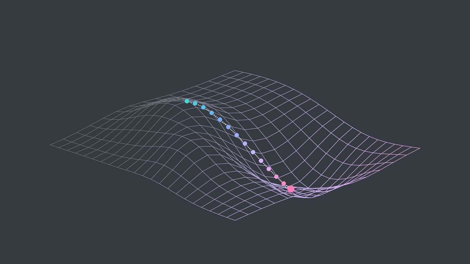
Why it matters: A production path for a well-understood problem class: define the problem once, let the mapper handle the translation to a quantum-ready Hamiltonian, and skip the error-prone manual encoding. More optimization tools are on the way.

Get started: Install with pip install qiskit-addon-opt-mapper, work through the how-to guides on GitHub, from defining a problem to converting and validating it, and learn how to map an optimization problem to a quantum circuit with the optimization mapper in our warm-start QAOA tutorial.

Code: Define an optimization problem, then convert it to a QUBO and map it to an Ising Hamiltonian ready for quantum execution.

from qiskit_addon_opt_mapper import OptimizationProblem
from qiskit_addon_opt_mapper.converters import OptimizationProblemToQubo
from qiskit_addon_opt_mapper.translators import to_ising

# Define the problem: variables, objective, constraints
mod = OptimizationProblem("my problem")
mod.binary_var(name="x")
mod.integer_var(name="y", lowerbound=-1, upperbound=5)
mod.minimize(linear={"x": 1}, quadratic={("x", "y"): 2})
mod.linear_constraint(linear={"x": 1, "y": 2}, sense="<=", rhs=3)

# Convert to QUBO, then to an Ising Hamiltonian for quantum execution
qubo = OptimizationProblemToQubo(penalty=1e5).convert(mod)
hamiltonian, offset = to_ising(qubo)

IBM Quantum application functions

A category of functions within IBM Quantum Functions: research-backed, drop-in functions built by ecosystem partners across optimization, QML, chemistry, and PDEs. You pass a classical problem description and get a classical result back—the function handles mapping to circuits, running, and post-processing.

Why it matters: Drop-in capabilities for domain problems. No need to build every layer of the stack yourself, or even to write the quantum code.

Get started: Browse the full lineup in the IBM Quantum Functions catalog—including Qunova's HI-VQE chemistry solver, Q-CTRL's optimization and dynamics solvers, ColibriTD's QUICK-PDE, and Kipu Quantum's Iskay optimizer.Learn how to solve a hard optimization problem with a few lines of code in our Kipu Quantum Iskay Quantum Optimizer tutorial.

Code: Every application function follows the same pattern—load it from the catalog, pass a problem, and run. As an example, we’ll look at Kipu Quantum's Iskay Quantum Optimizer.

from qiskit_ibm_catalog import QiskitFunctionsCatalog

catalog = QiskitFunctionsCatalog()
optimizer = catalog.load("kipu-quantum/iskay-quantum-optimizer")

# Define the optimization problem as coefficients (QUBO/HUBO or spin format)
problem = {"()": 1, "(0,)": 1.5, "(1,)": 2}

job = optimizer.run(
    problem=problem,
    problem_type="spin",
    backend_name=backend_name,
    options={"shots": 5000, "num_iterations": 5},
)
result = job.result()

Getting hands-on after QDC

Using the latest quantum capabilities doesn't require special access or a large budget. Developers on the IBM Quantum Open Plan who use 20 minutes of runtime within any rolling 12-month period can request 180 minutes of access over 12 months, enabling more experimentation and longer-running workflows. And there are more ways to get involved:

• IBM Quantum Open Plan: free access, now expanded for active users.
• IBM Quantum Credits: apply for IBM-funded access to run larger workloads on real hardware.
• IBM Quantum Classroom Accounts: teaching and learning resources, plus shared accounts for classrooms and groups.
• Quantum Advantage Tracker: community tracker for measuring progress toward quantum advantage.